判别模型与生成模型
| Component | Supervised Learning | Unsupervised Learning |
|---|---|---|
| Data | (x: data, y: label) | (x: data) |
| Goal | learn a function to map x->y | learn some hidden structure of the data |
| Examples | Classification, Object Detection, Regression, Semantic Segmentation | Clustering, Dimensionality Reduction(e.g., PCA), Feature Learning |
一般来说,从学习概率分布的角度来说,模型可以分为三类。
判别模型Discriminative Model: Learn a probability distribution \(p(y|x)\)
生成模型Generative Model: Learn a probability distribution $p(x)$
条件生成模型Conditional Generative Model: Learn conditioned probability given label y \(p(x|y)\)
Note that probability density function $p(x)$ is normalized
$\int_X p(x)dx = 1$
Thus different values of $x$ compete for density
For discrimitive models, there are competitions for different labels, but no competition between images. Therefore, discrimitive models can’t handle unseen samples, the label distributions for all images must be given.
For generative models, all the images compete for probability mass. Therefore, the model can ‘reject’ unreasonable inputs by assigning low probability.
生成模型分类
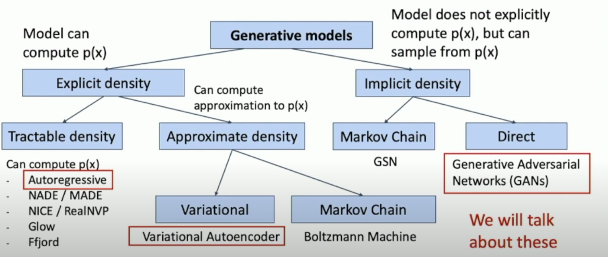
自回归模型Autoregressive Models
Explicit Density Estimation
**Goal: ** find an explicit function for $p(x)=f(x,W)$
Given the dataset $X(x^{(1)},x^{(2)},\dots,x^{(N)})$, train the model by solve:
\[\begin{align} W^*&=\arg \max_W\prod_i p(x^{(i)})\\ &=\arg \max_W\sum_i log\;p(x^{(i)})\\ &= \arg \max_W\sum_i log\;f(x^{(i)}, W) \end{align}\]This will maximize the probability of training data (i.e., Maximum Likelihood Estimation)
Autoregressive Models
Autoregressive models are concrete implements of the general analysis above.
-
Assume $x$ consists of multiple subparts
\[x=(x_1, x_2, \dots,x_T)\] -
Use chain rule to break down $p(x)$
\[\begin{align} p(x)&=p(x_1,x_2,\dots,x_T)\\ &=p(x_1)p(x_2|x_1)p(x_3|x_1,x_2)\dots\\ &=\prod_{t=1}^Tp(x_t|x_1,x_2,\dots,x_{t-1}) \end{align}\] -
Next subpart will rely on all the previous subparts $\rightarrow$ Recurrent Neural Network!
PixelRNN
PixelRNN从图像的左上角开始,逐步生成像素,左边和上方的像素就构成了previous subparts,因此,新的hidden state的计算就是 \(h_{x,y}=f(h_{x-1,y},h_{x,y-1},W)\) 对于每个像素,依次预测其R G B值: 即在[0, 1, .., 255]做一个softmax来选择概率最大的像素值。
PixelRNN可以横向和纵向来进行,示意图如下:
这种思路和实现方式非常简明,但缺点就是性能很差,一个$N\times N$的图像需要$2N-1$个时间步来完成,由于隐状态的依赖性所以并行性很差。
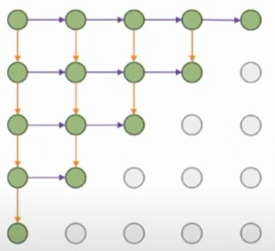
PixelCNN
一种改进思路就是,用类似卷积核的方式来生成当前像素的隐状态,例如下面这个示意图里,用*表示已经生成的像素,-表示未生成的像素,@表示当前正在生成的像素,+表示生成新像素时所使用的像素。
* * * * * * * * * * * * * *
* * * * * + + + + + * * * *
* * * * * + + + + + * * * *
* * * * * + + + + + * * * *
* * * * * + + + + + * * * *
* * * * * + + @ - - - - - -
- - - - - - - - - - - - - -
可以通过掩码遮挡未来信息的方式,来让模型在训练数据上进行并行卷积对像素做预测,从而提高训练效率。但并没有解决在测试时需要逐个计算像素的问题。
变分自编码器Variantial Autoencoders(VAE)
VAE中density function没有办法进行显式的计算和优化,而是针对其下界进行优化。
Regular Autoencoders
Unsupervised method for learning feature vectors from raw data.
The features extract useful information for downstream tasks.
Idea: Use encoder to extract the feature and use the features to reconstruct tthe input data with a decoder. The “Autoencoder” is encoder itself.
Loss: L2 distance between input and reconstructed data.
The encoder compress the input data to extract features which are lower dimentional than the data. After training, we only use the encoder for downstream tasks.
Variational Autoencoders
从上面可以看到Regular Autoencoder只是学习了如何提取数据的潜在特征以用于下流任务,但这其中没有能用于生成新图像的方式。
首先假设训练数据$x$是从目前未观测到的latent representation $z$来生成的,当模型训练完成后,我们可以从一个人为假设的先验分布$p_{\theta^*}(z)$中去采样新的$z$(e.g., Gaussian),然后将这个潜在特征输入到一个类decoder的结构中,来计算 \(p_{\theta^*}(x|z^{(i)})\) 从而得到新的数据的概率分布,这一结构就可以用一个神经网络来实现。
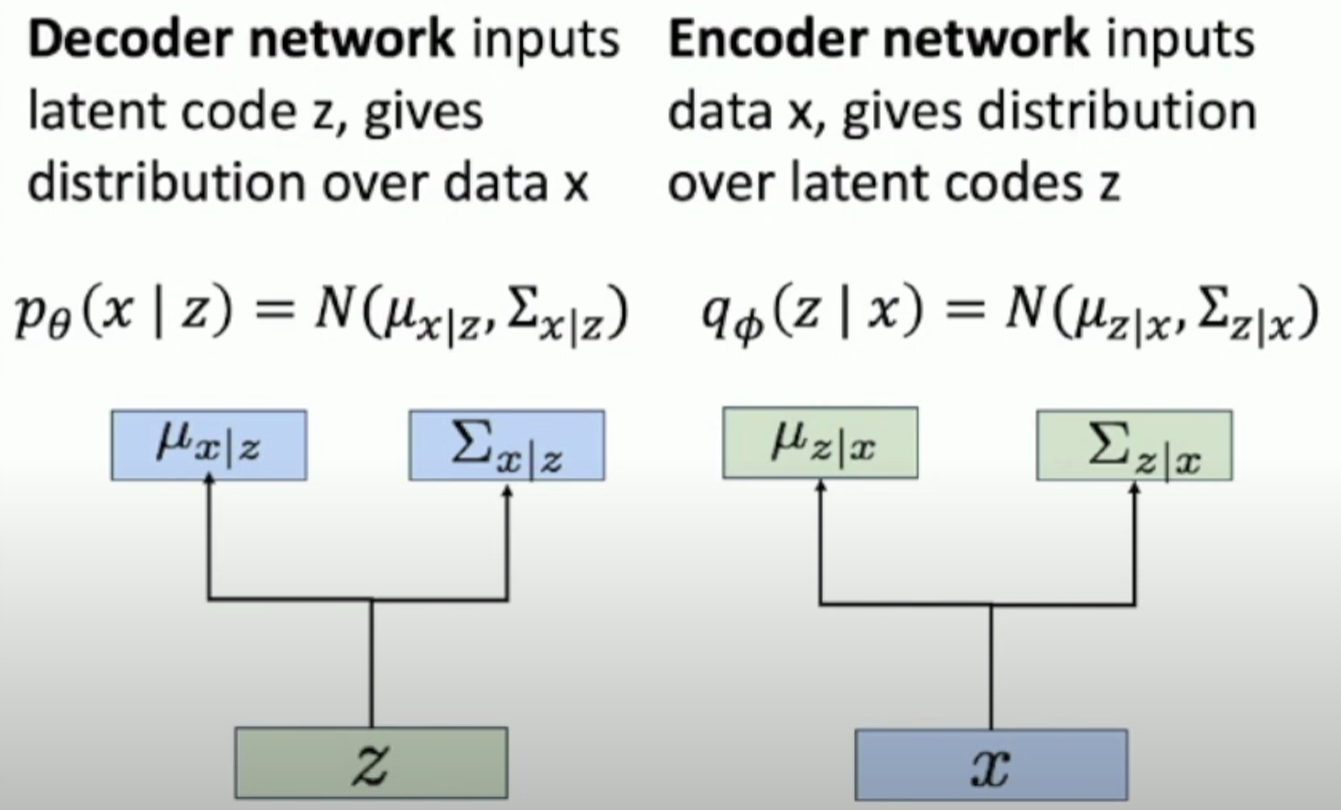
具体来说,相应的模型是通过输入潜在特征$z$,然后预测一个高维的高斯分布去表示上述概率分布,高斯分布的维度即图像中的像素数量,均值表示每个像素的均值,协方差表示的是每个像素上的协方差。
How to train?
如果说训练时可以观测到每个数据x对应的潜在特征表示z的话,是可以直接作为条件生成模型去训练了,但事实上没有办法观测到z。所以我们采用Bayes法则去计算,这里我们注意到,$p_{\theta}(x|z)$就是decoder的预测结果,是可知的;$p_{\theta}(z)$是一个先验分布,也是可知的;但问题是$p_{\theta}(z|x)$是没有办法用当前这个模型来找到的,因此我们可以另外训练一个Encoder用来预测给定输入图像$x$时的潜在特征的概率分布$q_{\phi}(z|x)$来作为近似,最终得到 \(p_{\theta}(x)=\frac{p_{\theta}(x|z)p_{\theta}(z)}{p_{\theta}(z|x)}\approx \frac{p_{\theta}(x|z)p_{\theta}(z)}{q_{\phi}(z|x)}\) VAE的架构如图所示:
接下来是要考虑训练时应该最大化什么参量。
先做一步恒等变换: \(\log p_{\theta}(x)= \log \frac{p_{\theta}(x|z)p(z)}{p_{\theta}(z|x)}=\log \frac{p_{\theta}(x|z)p(z)q_{\phi}(z|x)}{p_{\theta}(z|x)q_{\phi}(z|x)}\\\)
然后引入期望来做替换 \(=E_z[\log p_{\theta}(x|z)]-E_z[\log \frac{q_{\phi}(z|x)}{p(z)}]+E_z[\log \frac{q_{\phi}(z|x)}{p_{\theta}(z|x)}]\\\)
再将后面两项替换为KL散度来表达 \(=E_{z\sim q_{\phi}(z|x)}[\log p_{\theta}(x|z)]-D_{KL}(q_{\phi}(z|x),p(z))+D_{KL}(q_{\phi}(z|x),p_{\theta}(z|x))\)
第一项反映的是图像重建,第二项反映的是先验分布和Encoder采样之间的KL散度,但第三项是没法计算的(之前所说的$p_{\theta}(z|x)$是无法观测的),因为KL散度一定非负,所以可得Variantional lower bound: \(\log p_{\theta}(x) \ge E_{z\sim q_{\phi}(z|x)}[\log p_{\theta}(x|z)]-D_{KL}(q_{\phi}(z|x),p(z))\)
Encoder和Decoder的训练目标就是最大化这一下界。