UMich DL for CV

Attention

Machine Translation (seq2seq)

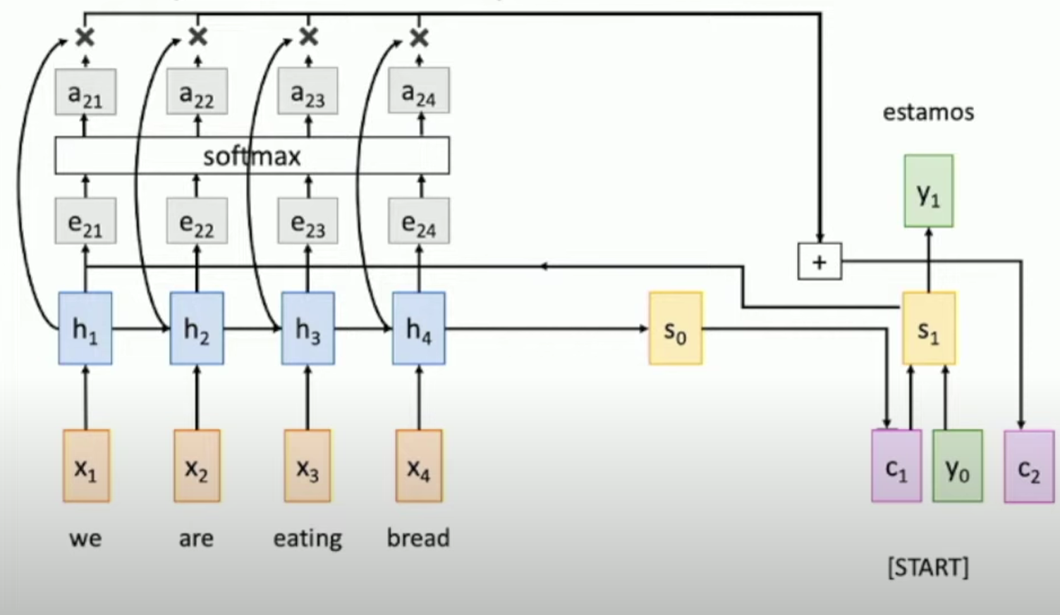
Here $a_{ij}$ represents the weights of input sequence predicted by the attention.

e.g., if the word ‘estamos’ = ‘eating’, then maybe $a_{23}=0.8\;a_{21}=a_{24}=0.05\;a_{22}=0.1$

Image Captioning

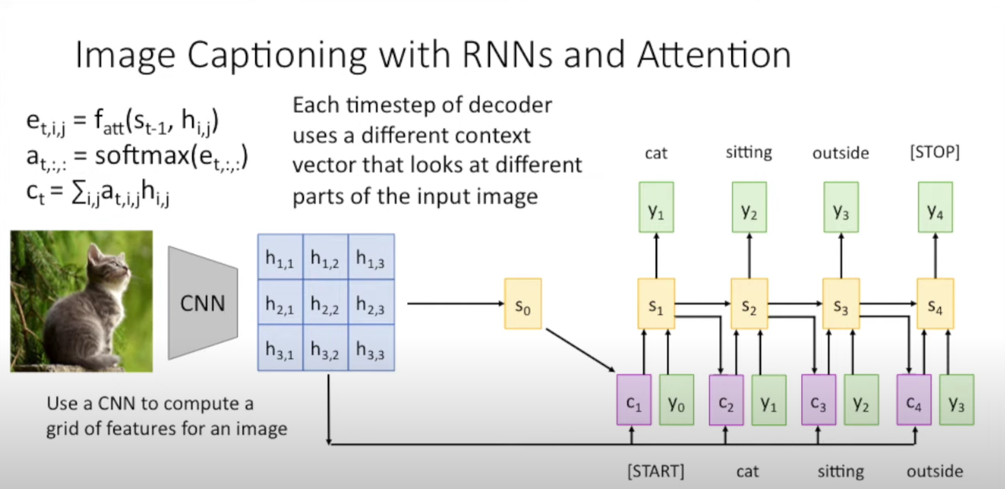
The output of the final Conv layers can be interpreted as a grid of feature vectors( $h_{i,j}$ in the image). Then use this grid to predict the initial hidden state $s_0$ for decoder RNN.

$e_{t,i,j}$ represents the alignment scores. The scalar is high when we want to put high weight on that part of the vector. Then we use softmax to normalize the alignment scores to produce the attention weights.

Generalize Attention

General form

Now let’s abstract and generalize this process for a general purpose layer.

Input

Query vector: $q$, shape: $(D_Q,)$, e.g., the hidden state vector at each timestep.

Input vector: $X$, shape: $(N_X,D_X)$, e.g., the feature vectors we want to attend over.

Similarity function: $f_{att}$

Computations

Similarity: $e$, shape: $(N_X,)$, $e_i = f_{att}(q, X_i)$

Attention Weights: $a=softmax(e)$, shape: $(N_X,)$

Output vector: $y= \sum_i a_i X_i$, shape: $(D_X, )$

Self-Attention Layer

Changes

• Replace the $f_{att}$ with scaled dot product $\rightarrow$ $e_i = \Large \frac{q \cdot X_i}{\sqrt{D_Q}}$
• Use multiple query vectors $Q$, shape $(N_Q,D_Q)$, $E=QX^T,A=softmax(E,dim=1),Y=AX$

Here we notice that we use the input vector $X$ in two ways : calculate the similarity $E$ and the ouput $Y$, to serve these different functions, we separate the input vector into 2 learnable matrices: Key Vector(for attention) and Value Vector(for output).

The new form looks like:

new input

Query vectors: $Q[N_Q,D_Q]$

Input vectors: $X[N_X,D_X]$

Key matrix: $W_K[D_X,D_Q]$

Value matrix: $W_V[D_X,D_V]$

new computation

Key vectors: $K[N_X, D_Q]=XW_K$

Value vectors: $V[N_X,D_V]=XW_V$

Similarities: $E[N_Q,N_X]=QK^T, E_{i,j}=Q_i\cdot K_j/ \sqrt{D_Q}$

Attention weights: $A[N_Q, N_X] = softmax(E,dim=1)$

Output vectors: $Y[N_Q,D_V]=AV\;Y_i=\sum_j A_{i,j}V_j$

For Self-Attention Layer, query vectors $Q$ is generated by input with Query matrix $W_Q$, that’s $Q=XW_Q$. The whole process looks like:

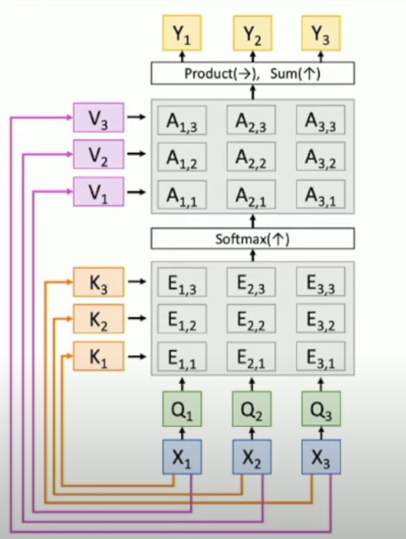
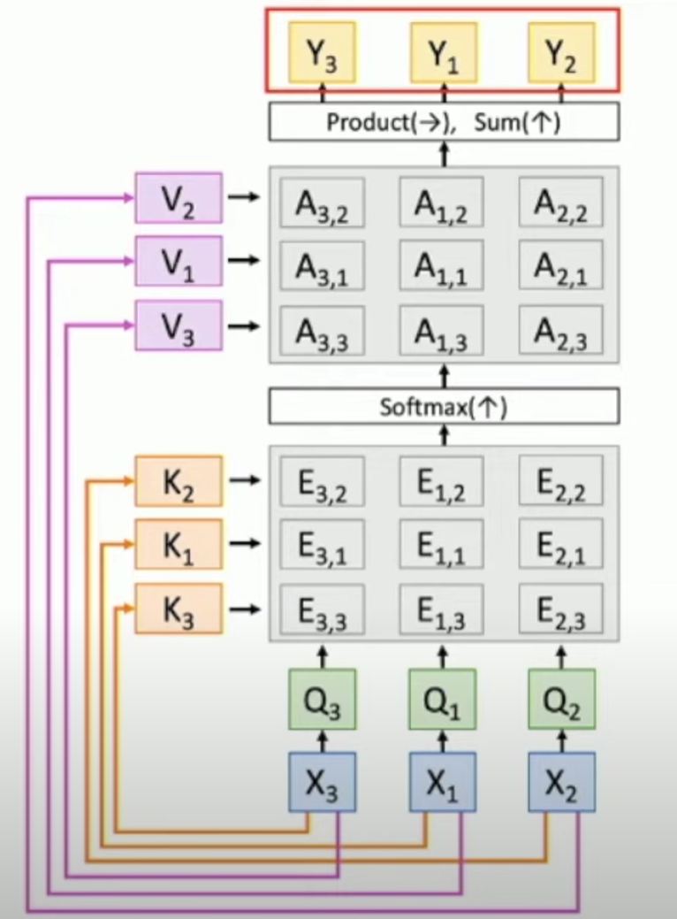
Permutation Equivariant

Here is a question: what happens when we permute the input (i.e., change the order of input)?

Answer: The output will be the same but also permuted. Which means the self-attention layer is Permutation Equivariant (i.e., f(g(x)) = g(f(x)) ), the process looks like:

Positional Encoding

So self-attention layer can’t tell the order of the vectors. But in some situations, we need the model to be aware of the positions of the vectors. Thus we introduce Positional encoding. For each input vector, give it an embedding vector to indicate its position. The construction of the embedding vectors is explicitly explained here.

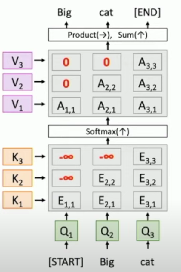
Masked Self-Attention Layer

Another variant is Masked Self-Attention Layer.

For normal self-attention layer, the model can access all the input information. However, sometimes we want the model only to use the information from the past, especially for language models.

To achieve this, we can simply change the $E$ value to $-inf$ in every position we don’t want the model to pay attention to.

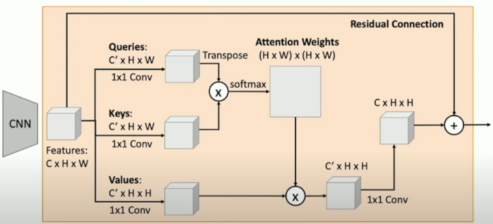
Example

Here is an example for CNN with Self-Attention:

Three ways of processing sequences

RNN

For Ordered Sequences

1D Conv

For Multidimensional Grids

Self-Attention

For Sets of vectors

The Transformer Block

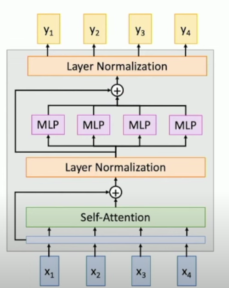
Input: Sets of vectors x

Output: Sets of vectors y

Self-Attention is the only interaction between vectors, LayerNorm and MLP work independently per vector.

A Transformer includes several Transformer blocks.

• Previous
  UMich DL for CV
• Next
  UMich DL for CV