Challenges
细粒度划分 Fine-grained Categories
例如猫的具体种类,缅因猫,布偶猫
背景杂乱 Background Clutter
动物可能具有的保护色,黑猫的深色背景,雪地里的北极狐,落叶堆里的橘猫
光照变换 Illumination Changes
光暗场景的Robustness
物体变形 Deformation
物体的形态发生变化,猫从蜷缩变为平躺
物体遮挡 Occlusion
只能够获取到目标的一部分,例如被毯子包住的猫
### Image Classification
最基本的分类思想:K-Nearest Neighbors
数据集划分为Train, Validation, Test三部分,Train部分用于训练kNN模型,记忆图像和labels;Validation部分用于选择超参数k;Test部分用于最终评估模型性能。
此外还有Cross Validation思想:将数据集分为若干个子集,每一轮中,这些子集轮流作为验证集合,其余的子集作为训练集。
Linear Classification
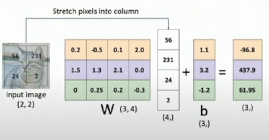
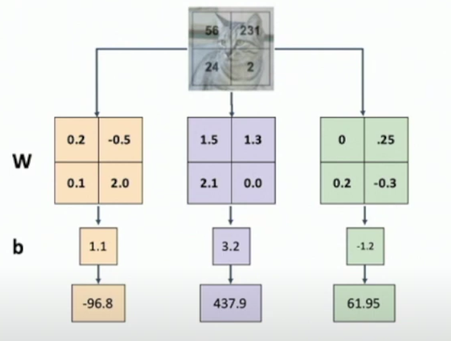
Algebraic Viewpoint
f(x, W) = Wx+b,W为权重矩阵,x是图像张成的向量,b是偏差bias
Visual Viewpoint
each row as one “template” for each category
但单个template无法捕捉到图像数据的不同模式(e.g. 位置和方向的变换)
Geometric Viewpoint

根据不同值的像素数量来确定不同类别的得分,在高维空间里形成相应的超平面
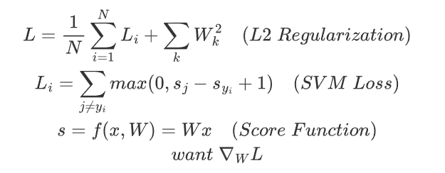
Loss Model
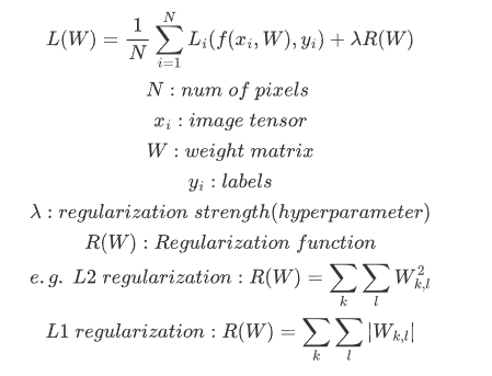
这里的Regularization的作用是为了防止模型过拟合训练集,如果模型overfitting,那么对于训练集上一些很小的扰动,模型都会刻画相应的权重特征,这就会导致权重矩阵的值增大,因此Loss Model中采用这种方式来作为惩罚项,避免模型过拟合。
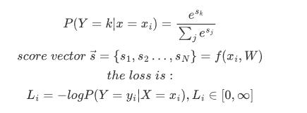
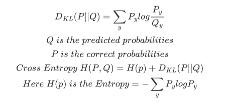
Cross-Entropy Loss
interpret the raw classifier scores as probabilities
for examples, scores:
3.2 5.1 -1.7
since probabilities must >= 0, we use an exponential function to give the unnormalized probabilities:
24.5 164.0 0.18
moreover, probabilities must sum to 1, so normalize:
0.13 0.87 0.00
The process can be done by Softmax
take the class corresponding to 0.13 as the correct class, then the loss is:
-log(0.13) = 2.04
the correct probabilities :
1.00 0.00 0.00
use Kullback-Leibler divergence to compare the two probabilities:
Optimization
Target
Find the w* = argmin_w {L(w)}
we notice that loss is a function of W:
Gradient Descent
# Vanilla Gradient Descent
w = init_weights()
for t in range(num_steps):
	dw = compute_grad(loss_fn, data, w)
	w -= learing_rate * dw
So here are 3 hyperparameters:
- Weights initialization method
- Number of steps
- Learning rate
Stochastic Gradient Descent (SGD)
# Stochastic Gradient Descent
w = init_weights()
for t in range(num_steps):
	minibatch = sample_data(data, batch_size)
	dw = compute_grad(loss_fn, minibatch, w)
	w -= learning_rate * dw
Since full sum is expensive, SGD approximates the sum using a minibatch of the whole data.
Here are 5 hyperparameters:
- Weight initialization method
- Number of steps
- Learning rate
- Batch size
- Data sampling method
SGD + Momentum
Momentum uses the previous gradient infomation to help speed up the convergence of SGD and reduce oscillations.
# SGD + Momentum
v = 0
for t in range(num_steps):
	dw = compute_grad(w)
	v = rho * v + dw
	w -= learning_rate * v
When the current gradient direction is the same as the previous, momentum accelerates the update.
When the current gradient direction is opposite, momentum slows down the update, thus reducing the oscillations.
Rho represents the “friction”, usually 0.9 or 0.99.
# equivalent form of SGD + Momentum
v = 0
for t in range(num_steps):
	dw = compute_grad(w)
	v = rho * v -  learning_rate * dw
	w += v
Nesterov Momentum
v = 0
for t in range(num_steps):
	dw = compute_grad(w)
	old_v = v
	v = rho*v - learning_rate *dw
	w -= rho*old_v - (1 + rho)*v
AdaGrad
grad_sqr = 0
for t in range(num_steps):
	dw = compute_grad(w)
	grad_sqr += dw*dw
	w -= learning_rate * dw / (grad_sqr.sqrt() + 1e-7)
AdaGrad introduces “Adaptive Learning Rates” or “Per-paramter learning rates” by adding element-wise scaling of the gradient based on the historical sum of squares in each dimension.
When the gradients changing very fast (steep direction, larger grad_sqr), the progress is damped.
When the gradients changing very slow (flat direction, smaller grad_sqr), the progress is accelerated.
Problem!
the grad_sqr will continue increasing! Finally w changes very very slow, the training is nearly stopped before getting to the optimal.
Thus we introduce : RMSProp (Leak AdaGrad)
RMSProp
grad_sqr = 0
for t in range(num_steps):
	dw = compute_grad(w)
	grad_sqr = decay_rate * grad_sqr + (1 - decay_rate) * dw * dw
	w -= learning_rate * dw /(grad_sqr.sqrt() + 1e-7)
we use decay_rate to solve the problem above, prevent grad_sqr from being too large.
Adam : RMSProp + Momentum
mmt1 = 0
mmt2 = 0
for t in range(num_steps):
	dw = compute_grad(w)
	mmt1 = beta1 * mmt1 + (1 - beta1) * dw
	mmt2 = beta2 * mmt2 + (1 - beta2) * dw * dw
    # Bias Correction
    mmt1_unbias = mmt1 / (1 - beta1 ** t)
    mmt2_unbias = mmt2 / (1 - beta2 ** t)
    # Bias Correction
	w -= learning_rate * mmt1_unbias / (mmt2_unbias.sqrt() + 1e-7)
mmt1代表了SGD+Momentum的idea
mmt2则代表了RMSProp的idea
由于两者初始化为0,就会导致第一次更新时,分母上是一个接近0的值。为了避免这一问题,引入了Bias Correction方法。假设beta1=0.9 beta2=0.999 dw=0.1
则mmt1 = 0.9 * 0 + 0.1 * 0.1 = 0.01
mmt2 = 0.999 * 0 + 0.001 * 0.1 * 0.1 = 0.00001
如果不进行修正,估计偏差带来的影响会非常大,影响我们的训练效果。
而在修正之后的结果就更加合理:
mmt1_unbias = 0.01 / (1 - 0.9^1) = 0.1
mmt2_unbias = 0.00001 / (1 - 0.999^1) = 0.01